Concepts

This page describes what SmartCer exposes: names, shapes, arguments and defaults. The physical and methodological background follows Stentati et al. (2022) and Guiducci et al. (MECO 2023).

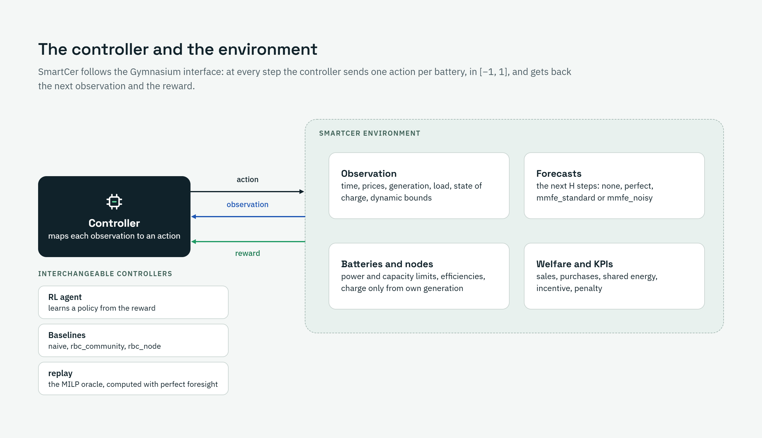
The controller loop.

The community

A community is a set of nodes of three types: producer, consumer and prosumer. Each node has hourly (or sub-hourly, delta_t) series of generation, load, sell price and buy price, and may have a battery (storage) and a photovoltaic plant (photovoltaic). At every step the environment computes the energy balance of each node, the energy fed into the grid and taken from it, the shared energy of the community (the minimum between total export and total import), the incentive on it (uniform, or tip, the Italian tariffa incentivante premio) and the social welfare: sales, minus purchases and storage costs, plus the incentive.

The agent controls the batteries only. Scenarios are folders read by smartcer.data.load_scenario; see Quickstart for an example.

How the community is modelled

SmartCer models a renewable energy community under the Italian virtual scheme. Members keep their own meters and supply contracts, and no energy is routed between them: at every step each node exchanges energy with the public grid at its own sell and buy prices. The community is then credited for the shared energy: the energy fed into the grid by its members that, in the same step, is matched by energy taken from the grid by other members. This is why shared energy is the minimum between total export and total import, and why it depends on when energy is exported, not only on how much.

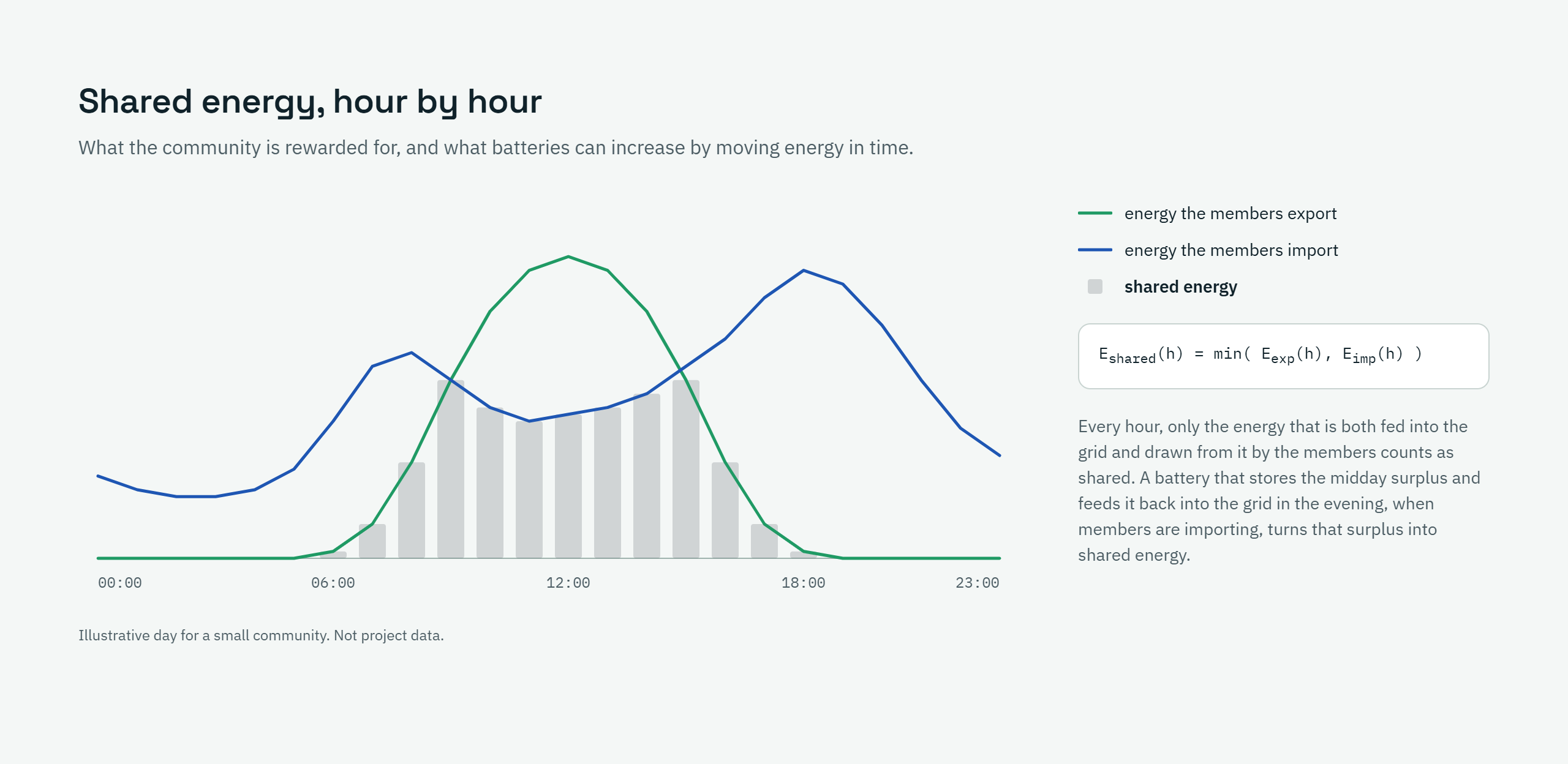
Shared energy is the minimum between total export and total import at every step (illustrative day).

The incentive rewards that coincidence. With the uniform model every kWh of shared energy earns the same unit value π^inc, as in the reference papers and in the MILP oracle; with tip it follows the per-plant premium tariff of the Italian rules (formulation, section 9).

Batteries are the only lever. A battery charges only from its own node’s generation (by default up to the generation of the step, charge_limit: production), never from the grid. Its state of charge follows the dynamics of Stentati et al. (2022): the power limits apply on the node side, the efficiencies between node and cell, and the state of charge stays between S^min and S^max. A battery can raise the welfare in two ways: it moves its node’s surplus to the steps in which the node would import, cutting purchases, and it moves exports to the steps in which other members import, increasing the shared energy and the incentive. The welfare W_t is the sum of the members’ sales minus their purchases and storage usage costs, plus the incentive: the quantity the MILP oracle maximises and the default reward.

Environment

gym.make('SmartCer-v1', scenario=..., **options) or smartcer.gym.SmartCerEnv directly. The main options and their defaults:

Argument	Default	Meaning
scenario	required	scenario folder (or a loaded Community)
start, end	None	period of the data to use
episode_length	None	steps per episode; None uses the whole period
random_start	False	random first step of each episode
observe_current_step	True	False observes generation and load of step t - 1 (causal timing)
observation	'meco'	observation preset: 'meco' or 'extended'
lookback	0	past steps of generation and load, 'extended' only
normalizer, normalizer_window	None	min-max bounds: a saved file, or the window to fit them on
reward	'welfare'	reward type: 'welfare', 'profit' or 'energy'
reward_per_node	False	per-node reward instead of the collective one
penalty_coefficient	10.0	weight σ of the constraint penalty
forecast	None	forecast provider name, see below
forecast_horizon	0	number of forecast steps H
oracle	None	folder of MILP oracle files
seed	None	seed

reset(seed) returns (obs, info); step(action) returns (obs, reward, terminated, truncated, info). terminated is always False: an episode ends with truncated=True on its last step.

Action space

Box(-1, 1, (N,), float32): one value per battery, N being the number of nodes with a battery, in the order of env.unwrapped.storage_node_ids. A positive value charges the battery, a negative one discharges it. Actions are clipped to [-1, 1] without penalty. The dynamic bounds of each battery, a_lower and a_upper, are part of the observation; the part of an action beyond them is clipped and enters the penalty K_t.

Observation space

A flat Box. env.unwrapped.obs_layout maps each feature name to its slice. Generation and load are min-max scaled with a MinMaxNormalizer and clipped to [0, 1]; info['obs_clipped'] counts the clipped values.

Presets (observation=):

• meco: time/month and time/hour (sine and cosine), time/day_of_week (one-hot); prices (price/sell and price/buy if all nodes share them, else <node>/sell_price and <node>/buy_price per battery node); per battery node <node>/generation, <node>/load, <node>/soc, <node>/a_lower, <node>/a_upper.

• extended: the same, plus time/holiday (Italian national holidays), community/generation and community/load (totals of the nodes without a battery) and, with lookback L, <node>/generation_lookback and <node>/load_lookback (L values each, most recent first).

Forecasts add a forecast section, see below.

Reward

R_t = M_t - σ K_t, with σ = penalty_coefficient. Options of reward:

reward	Main term M_t
'welfare' (default)	community social welfare W_t; collective only
'profit'	revenue minus cost minus storage cost per node; the collective variant adds the incentive
'energy'	minus the squared energy imported by each node (legacy of version 0.6.2)

With reward_per_node=True the reward is computed per battery node, r_u = m_u - σ k_u, and R_t is their sum; the per-node values are in info['reward']['nodes']. It is not available for 'welfare'. The components of every step are in info['reward'] (type, main, penalty, total).

Forecasts in the observation

With forecast and forecast_horizon H the observation contains H future values, ordered by lead time, of: the sale price (exact), the generation and load of every battery node, and the totals of the nodes without a battery. There are four settings of forecast:

• None (default): no forecast. The agent observes only the current step. This is the baseline of the MECO 2023 paper.

• 'perfect': the true future values.

• 'mmfe_standard': simulated forecast errors, standard preset.

• 'mmfe_noisy': simulated forecast errors, larger preset.

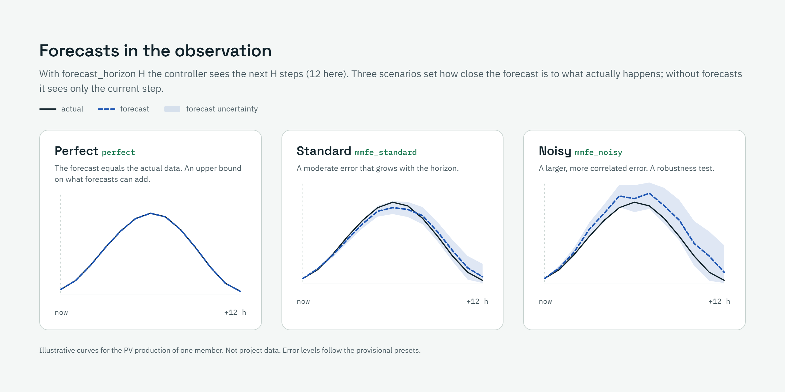
Forecast scenarios (illustrative curves).

The three forecast scenarios are perfect, mmfe_standard and mmfe_noisy. mmfe_perfect is also registered: the MMFE provider with zero error, useful to check that MMFE and perfect give the same forecast observations.

env = gym.make('SmartCer-v1', scenario='path/to/scenario',
               forecast='mmfe_standard', forecast_horizon=12)

The MMFE providers (smartcer.forecasts.MMFEForecast) add errors with the martingale model of forecast evolution: the innovations of each target step are drawn once per episode, so the error variance grows with the lead time. The preset parameters are provisional:

Preset	sigma_generation	sigma_load	rho	phi
standard	0.07	0.03	0.5	0.8
noisy	0.15	0.08	0.7	0.9

Custom parameters: build MMFEForecast(community, MMFEParameters(...)) and pass the object as forecast. info['privileged']['true_future'] holds the true values of the forecast steps, for a critic that is allowed to see them.

Why the martingale model

Simulated forecasts must not be easier to use than real ones. Independent noise at every step and node would make them easier in three ways: the agent could average the errors of adjacent steps, the errors of different plants would cancel in the community total, and the forecast of the same step would jump from one issue to the next. The martingale model of forecast evolution (Heath and Jackson, 1994) avoids all three. For each target step the innovations of all lead times are drawn once: the forecast issued h steps ahead carries h of them, so its error variance grows linearly with h, and each new step reveals one more, so successive forecasts of the same target converge consistently to the true value.

rho and phi set the correlation of the errors. rho is the share of the error that is common to all series of the same quantity: the photovoltaic plants of a community share the weather, so with a high rho an over-forecast of one plant comes with an over-forecast of the others and the errors do not cancel in the total. phi is the persistence of that common error over consecutive target steps: an afternoon cloudier than forecast is wrong for several hours in a row, not for one. Two series of the same quantity have error correlation rho; two adjacent target steps of one series have correlation rho·phi. The presets have no systematic error; a bias can be added with bias_generation and bias_load. All parameters are described in the configuration reference (Forecasts).

MILP oracle

An optional folder of optimal battery trajectories computed by a MILP, passed as oracle=. The file format is provisional:

oracle/
├── trajectory.csv   # datetime, node_id, p_cha_kw, p_dis_kw, soc_kwh: one row per step and battery
└── objective.csv    # optional: date, objective (welfare of the day, EUR)

With an oracle:

• info['privileged'] holds oracle_action and oracle_soc, for the critic of an asymmetric actor-critic; they never enter the observation.

• The replay controller plays the optimal actions.

• smartcer.gym.controllers.check_replay(env, output_dir) plays them over whole days and checks that no step is penalised and that the cumulative welfare is within a relative tolerance (default 1e-3) of the MILP objective. It writes oracle_daily.csv and oracle_replay.json.

• The tracker adds the gap between the agent’s and the oracle’s state of charge to the battery tables and KPIs.

The initial state of charge inferred from the first row of the oracle file must match the one of the scenario.

What the oracle is

SmartCer does not solve the MILP: it reads a trajectory computed outside it. The oracle is the solution of the optimisation problem of Stentati et al. (2022) on the same model as the environment, solved with perfect knowledge of generation, load and prices: maximise the cumulative social welfare over the horizon, subject to the battery dynamics and bounds, the charge rule and the node balances. A binary variable keeps a node from exporting and importing in the same step; the minimum in the shared energy is replaced by an auxiliary variable bounded by total export and by total import, which the maximisation pushes to the minimum. The oracle files can come from any MILP on this model. A whole year can be solved over rolling windows (for example 48 h, keeping the first 24 h), so that the batteries are not emptied artificially at the end of each window; the MECO 2023 study instead imposed empty batteries at every day boundary, a constraint SmartCer does not model (formulation, section 14).

Because it knows the future, the oracle is the practical upper bound of a controller that does not: it is exact only when the MILP solves the same model as the environment over the whole period. With extra constraints, such as empty batteries at the end of each day, or with rolling windows, a controller can occasionally do better. It has two uses: a reference for comparisons (cumulative welfare, Fit Score) and privileged information for training, where an asymmetric actor-critic gives the oracle action to the critic only (Guiducci et al., MECO 2023). The replay check is what makes both uses valid: if the environment replays the MILP trajectory without penalties and reproduces its objective, the two share the same model.

Baselines

Controllers available in smartcer.gym.controllers.CONTROLLERS:

Name	Behaviour
naive	zero action on every battery: the batteries stay idle (self-discharge only)
rbc_community	rule-based controller, community mode: the same fraction of every battery’s charge (discharge) capacity, from the energy balance of the community
rbc_node	rule-based controller, node mode: each battery follows the balance of its own node
replay	the oracle actions; needs an environment with oracle=

naive is the “no storage control” baseline: there is no separate controller that removes the batteries from the community. The rule-based controllers are Algorithm 1 of the MECO 2023 paper; their actions always lie within the dynamic bounds.

compute_baselines(env, output_dir, controllers=('naive', 'rbc_community'), seed=None) runs controllers over the same episode and writes their results, see KPIs and outputs. run_episode(env, controller, seed) runs a single one.

Reading the baselines

naive measures what the community earns with idle batteries: every controller should be compared with it. The rule-based controllers react only to the current balance, without prices or forecasts. rbc_community charges when the community as a whole has a surplus and discharges when it has a deficit, sharing the energy among the batteries in proportion to what each can take or deliver in the step; rbc_node does the same with each node’s own balance. Both stay within the dynamic bounds, so they are never penalised. They are references, not lower bounds: a myopic rule can do worse than idle batteries. rbc_node, for example, stores its node’s surplus even when other members are importing, and so removes energy that would have been shared.

The Fit Score compares the daily welfare of a controller with that of the oracle and reads like a coefficient of determination: 100 means the same welfare as the oracle on every day, 0 means that the controller follows the oracle no better than a constant equal to the oracle’s mean daily welfare, and it is negative when it does worse. It complements the cumulative welfare: two controllers with the same yearly welfare can follow the oracle very differently day by day.